PowerGridPlanning.jl Tutorial

Wildfire-Informed Transmission Switching and Infrastructure Planning

This tutorial walks through the core features of PowerGridPlanning.jl: optimal transmission switching (OTS) under wildfire risk, infrastructure investment planning (hardening, batteries, solar), plotting, and nonlinear AC verification. We use the RTS-GMLC (73-bus) network and the bundled test_data/ reference dataset throughout, so every cell runs on a fresh clone with no downloads.

Docs page and notebook are the same document

This page and the repository's tutorial.ipynb are both generated from a single Literate.jl source (docs/lit/tutorial.jl), and the code below is executed when the documentation is built — the outputs you see are real.

1. Setup

Install the package (and HiGHS, used as the solver here) from the Julia REPL:

using Pkg
Pkg.add(["PowerGridPlanning", "HiGHS", "CSV", "DataFrames", "Plots", "JLD2"])

If you are running the notebook from a clone of the repository, activate the project environment instead:

using Pkg
Pkg.activate(".")     # from the repository root
Pkg.instantiate()

using PowerGridPlanning
using HiGHS
using CSV, DataFrames, Plots, Printf

Planning solves default to Gurobi, which requires a license. Throughout this tutorial we pass :optimizer => HiGHS.Optimizer so everything runs with the open-source HiGHS solver instead; if you have Gurobi, simply drop that entry. We also shorten the planning horizon to the first 6 hours of each day (:T => 6) to keep every solve fast — set :T => 24 (the default) for full-day studies.

SETTINGS = Dict(
    :data_dir  => "test_data",         # bundled reference dataset (resolved from the package root)
    :optimizer => HiGHS.Optimizer,     # open-source solver; remove to use Gurobi
    :silent    => true,                # suppress the solver's own log output
    :T         => 6,                   # hours per day (24 for full-day studies)
);

2. Data Overview

The repository ships with test_data/, a reference subset covering June 2020 for all six pre-configured networks (June 2021 for RTS). It includes network case files, per-line wildfire risk (USGS Fire Potential Index), bus coordinates, solar capacity factors, and basemap shapefiles.

DATA = joinpath(pkgdir(PowerGridPlanning), "test_data")
foreach(d -> println("test_data/", d, "/"), readdir(DATA))

test_data/CATS/
test_data/USGS_FPI/
test_data/US_Shapefiles/
test_data/bus_lat_lons/
test_data/census_data/
test_data/networks/
test_data/solar_data/

Wildfire risk is stored per (line, day). Here are the first rows of the RTS risk file:

rts_risk = CSV.read(joinpath(DATA, "USGS_FPI", "RTS", "2020_risk.csv"), DataFrame)
first(rts_risk, 5)

5×9 DataFrame

Row	date_of_forecast	date_of_risk	branch_id	max_wfpi	mean_wfpi	cum_wfpi	hr_max_wfpi	hr_mean_wfpi	hr_cum_wfpi
	Date	Date	Int64	Int64	Float64	Int64	Int64	Float64	Int64
1	2020-06-04	2020-06-04	1	0	0.0	0	0	0.0	0
2	2020-06-04	2020-06-04	2	112	103.455	2276	112	78.0455	1717
3	2020-06-04	2020-06-04	3	108	100.4	2008	108	62.4	1248
4	2020-06-04	2020-06-04	4	107	100.571	704	107	75.1429	526
5	2020-06-04	2020-06-04	5	110	102.522	2358	110	73.5652	1692

Time specification

The :times parameter accepts several formats:

:times => [(2020, 6, 15)]                    # single day
:times => [(2020, 6, 10), (2020, 6, 15)]     # specific days
:times => "June 2020"                        # full month
:times => "2020"                             # full year

3. Basic Optimizations

We solve three variants and compare them side by side:

Run	Model	Entry point	Objective	Switching	What it represents
A	DCOPF	`solve_opf`	`loadshed`	disabled	True no-action baseline
B	DCOTS	`solve_ots`	`loadshed`	thresholded	Fast heuristic: pre-remove riskiest lines
C	DCOTS	`solve_ots`	`tradeoff`	optimal	Full MIP: co-optimize shed and risk

3a. Baseline DCOPF (no switching)

DCOPF is a pure power-flow model. Use solve_opf for OPF baselines: no switching variables and no wildfire risk enter the mathematical model at all.

results_base = solve_opf(merge(SETTINGS, Dict(
    :network   => "RTS",
    :model     => "DCOPF",
    :objective => "loadshed",
    :times     => [(2020, 6, 15)],
)));

 Downloading artifact: powerio_capi
✓ OPF-only model (DCOPF): wildfire risk disabled
Building DCOPF model...
Switching method: optimal
Network: RTS
Objective: loadshed
Days: 1, Hours per day: 6
Adding variables...
Adding objective function...
Adding constraints...
Solving optimization...
Extracting results...
Optimization complete!
Status: OPTIMAL
Objective value: 0.0
Total load shed: 0.0
Risk reduction: 0.0%

3b. Thresholded switching (fast heuristic)

The thresholded method ranks risky lines and de-energizes the riskiest ones before solving, so the remaining problem is an LP. threshold_pct = 0.5 keeps at most 50% of the total wildfire risk energized.

results_thresh = solve_ots(merge(SETTINGS, Dict(
    :network          => "RTS",
    :model            => "DCOTS",
    :objective        => "loadshed",
    :times            => [(2020, 6, 15)],
    :switching_method => "thresholded",
    :threshold_pct    => 0.5,
)));

Loading RTS wildfire data from CSV...
Loaded RTS wildfire data from CSV for 1 days, max 90 risky lines per day
Converting threshold percentage 50.0% to absolute value: 103529.0
Total risk: 207058.0
Building DCOTS model...
Switching method: thresholded
Network: RTS
Objective: loadshed
Days: 1, Hours per day: 6

=== Computing Thresholded Line Statuses ===
Target threshold: 103529.0
Day 1: De-energized 16/90 risky lines
  Total risk: 207058.0
  Active risk: 102220.0
  Removed risk: 104838.0 (50.6%)
===========================================

Adding variables...
Adding objective function...
Adding constraints...
Solving optimization...
Extracting results...
Optimization complete!
Status: OPTIMAL
Objective value: 2.0821109759999987
Total load shed: 2.0821109759999987
Risk reduction: 50.63%
Total islanded buses: 4

3c. Optimal switching with the tradeoff objective

The tradeoff objective jointly minimizes load shedding and wildfire risk exposure; tradeoff_weight sets the balance (0 → pure load shed, 1 → pure risk).

results_opt = solve_ots(merge(SETTINGS, Dict(
    :network         => "RTS",
    :model           => "DCOTS",
    :objective       => "tradeoff",
    :tradeoff_weight => 0.5,
    :times           => [(2020, 6, 15)],
)));

Loading RTS wildfire data from CSV...
Loaded RTS wildfire data from CSV for 1 days, max 90 risky lines per day
Building DCOTS model...
Switching method: optimal
Network: RTS
Objective: tradeoff
Days: 1, Hours per day: 6
Adding variables...
Adding objective function...
Adding constraints...
Solving optimization...
Extracting results...
Optimization complete!
Status: OPTIMAL
Objective value: 0.05296252004420112
Total load shed: 14.084328960000056
Risk reduction: 95.02%
Total islanded buses: 61

Comparison

runs = [
    ("A: Base DCOPF",       results_base),
    ("B: Thresholded 50%",  results_thresh),
    ("C: Optimal tradeoff", results_opt),
]

println(@sprintf("%-20s  %12s  %10s  %10s", "Run", "Shed (MW)", "Risk red.", "Lines off"))
for (name, r) in runs
    println(@sprintf("%-20s  %12.2f  %9.1f%%  %10d",
        name, r[:total_load_shed], r[:risk_reduction_pct],
        length(r[:switched_off_lines][1])))
end

Run                      Shed (MW)   Risk red.   Lines off
A: Base DCOPF                 0.00        0.0%           0
B: Thresholded 50%            2.08       50.6%          16
C: Optimal tradeoff          14.08       95.0%          77

The de-energized line IDs are available per day:

println("Lines off (thresholded): ", results_thresh[:switched_off_lines][1])
println("Lines off (optimal):     ", results_opt[:switched_off_lines][1])

Lines off (thresholded): [12, 43, 46, 53, 54, 66, 67, 68, 72, 81, 83, 91, 92, 100, 101, 118]
Lines off (optimal):     [2, 3, 4, 5, 8, 12, 13, 14, 19, 20, 21, 24, 27, 28, 29, 31, 33, 34, 35, 40, 41, 42, 43, 44, 45, 46, 48, 49, 50, 52, 53, 54, 55, 60, 61, 62, 63, 66, 67, 68, 69, 71, 72, 73, 74, 75, 76, 78, 79, 81, 82, 83, 84, 85, 86, 87, 88, 90, 91, 92, 94, 96, 97, 99, 100, 101, 104, 105, 106, 108, 113, 114, 115, 116, 118, 119, 120]

Generation and load shedding over time

Result arrays have shape [D × T × units]. Summing over generators gives the hourly dispatch profile:

T = SETTINGS[:T]
gen(r) = [sum(r[:g][1, t, :]) for t in 1:T]

plot(1:T, [gen(results_base) gen(results_thresh) gen(results_opt)] .* 100,
     label=["Base DCOPF" "Thresholded" "Optimal tradeoff"],
     xlabel="Hour", ylabel="Total generation (MW)",
     marker=:circle, lw=2, legend=:bottomright)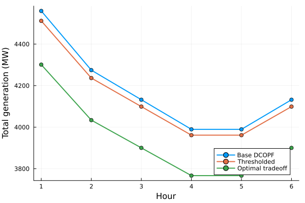

4. Infrastructure Investments

PowerGridPlanning co-optimizes operational switching with long-term investments, all sharing one :infrastructure_budget:

Line hardening — permanently reduce a line's wildfire risk (vegetation management, covered conductors, undergrounding)
Battery energy storage (BESS) — siting, sizing, and hourly dispatch
Solar PV — siting and sizing with hourly capacity factors

Investment variables are only added to the model when the corresponding feature is enabled.

4a. Line hardening

Here a risk constraint (threshold_pct) forces risky lines out of service — unless the budget hardens them, which lets them stay energized at reduced risk.

results_harden = solve_ots(merge(SETTINGS, Dict(
    :network                => "RTS",
    :model                  => "DCOTS",
    :objective              => "loadshed",
    :times                  => [(2020, 6, 15)],
    :threshold_pct          => 0.5,
    :hardening_enabled      => true,
    :hardening_cost_per_mile => 1e6,
    :infrastructure_budget  => 5e7,     # $50M shared budget
)));

println("Hardened lines: ", results_harden[:hardened_lines])
println("Load shed: $(round(results_harden[:total_load_shed], digits=2)) MW ",
        "(vs $(round(results_thresh[:total_load_shed], digits=2)) MW without hardening)")


--- Validating Hardening Parameters ---
✓ Hardening parameters validated:
  Effectiveness: 100.0% risk mitigation
  Cost per mile: $1.0M
  Infrastructure budget: $0.05B (shared)
  Enforce energization: true
Loading RTS wildfire data from CSV...
Loaded RTS wildfire data from CSV for 1 days, max 90 risky lines per day

--- Preparing Hardening Infrastructure ---
  Determined hardenable lines: 90 lines with wildfire risk

--- Line Length Data Summary ---
✓ Calculated line lengths for 120 lines
  Total network length: 3380.0 miles
  Lines with coordinates: 120 / 120

--- Hardening Budget Analysis ---
  Hardenable lines: 90
  Total hardenable miles: 2892.0
  Max hardening cost: $2.89B
  Budget allows: 1.7% of max hardening
Converting threshold percentage 50.0% to absolute value: 103529.0
Total risk: 207058.0
Building DCOTS model...
Switching method: optimal
Network: RTS
Objective: loadshed
Days: 1, Hours per day: 6
Adding variables...
✓ Added hardening variables for 90 lines
Adding objective function...
Adding constraints...
Setting risk threshold of 103529.0
Solving optimization...
Extracting results...
Optimization complete!
Status: OPTIMAL
Objective value: 0.9399999999999997
Total load shed: -2.7755575615628914e-16
Risk reduction: 50.81%
Total islanded buses: 2
Hardened lines: [42, 48, 55, 56, 71, 73, 74, 86, 94, 96, 120]
Load shed: -0.0 MW (vs 2.08 MW without hardening)

4b. Battery storage

With the tradeoff objective, the solver de-energizes risky lines and places storage where it best covers the resulting shortfalls.

results_batt = solve_ots(merge(SETTINGS, Dict(
    :network               => "RTS",
    :model                 => "DCOTS",
    :objective             => "tradeoff",
    :tradeoff_weight       => 0.5,
    :times                 => [(2020, 6, 15)],
    :battery_enabled       => true,
    :battery_cost_per_pu   => 1e7,      # $ per p.u. (100 MWh)
    :infrastructure_budget => 5e7,
)));

println("Buses with batteries: ", results_batt[:batteries_installed])


--- Validating Battery Parameters ---
✓ Battery parameters validated:
  Cost per p.u. (100MWh): $10.0M
  Charge efficiency: 95.0%
  Discharge efficiency: 95.0%
  SOC carryover: 99.9958%
  Charge rate: 1.0 p.u./hour
  Discharge rate: 1.0 p.u./hour
  Exclusive operation: false
  Infrastructure budget: $0.05B (shared)
Loading RTS wildfire data from CSV...
Loaded RTS wildfire data from CSV for 1 days, max 90 risky lines per day

--- Preparing Battery Infrastructure ---
  Battery candidates: 73 buses (all)
✓ Battery candidate buses identified: 73 buses
Building DCOTS model...
Switching method: optimal
Network: RTS
Objective: tradeoff
Days: 1, Hours per day: 6
Adding variables...
✓ Added battery variables for 73 candidate buses
Adding objective function...
Adding constraints...
Solving optimization...
Extracting results...
Optimization complete!
Status: OPTIMAL
Objective value: 0.04399279599001698
Total load shed: 9.334619375290762
Risk reduction: 95.02%
Total islanded buses: 61
Buses with batteries: [104, 204, 205, 208, 304, 305]

Dispatch profile of the largest installed unit:

batt_buses = results_batt[:batteries_installed]
if !isempty(batt_buses)
    bus = batt_buses[argmax([results_batt[:x][b] for b in batt_buses])]
    soc       = [results_batt[:soc][1, t, bus] for t in 0:T] .* 100
    discharge = [results_batt[:p_discharge][1, t, bus] for t in 1:T] .* 100
    charge    = [results_batt[:p_charge][1, t, bus] for t in 1:T] .* 100

    p1 = plot(0:T, soc, lw=2, marker=:circle, label="State of charge (MWh)",
              xlabel="Hour", legend=:best)
    p2 = bar(1:T, discharge .- charge, label="Net discharge (MW)", xlabel="Hour")
    plot(p1, p2, layout=(2, 1), size=(700, 500),
         plot_title="Battery at bus $bus ($(round(results_batt[:x][bus]*100, digits=1)) MWh)")
end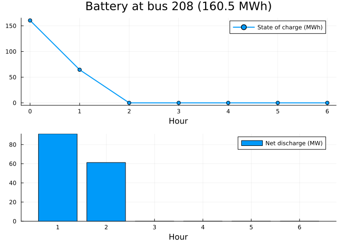

4c. Combined portfolio: hardening + batteries + solar

All three investment types compete for the same budget; the solver allocates spending across them optimally.

results_all = solve_ots(merge(SETTINGS, Dict(
    :network                => "RTS",
    :model                  => "DCOTS",
    :objective              => "tradeoff",
    :tradeoff_weight        => 0.5,
    :times                  => [(2020, 6, 15)],
    :hardening_enabled      => true,
    :hardening_cost_per_mile => 1e6,
    :battery_enabled        => true,
    :battery_cost_per_pu    => 1e7,
    :solar_enabled          => true,
    :solar_cost_per_pu      => 1e7,
    :solar_data_path        => joinpath(DATA, "solar_data", "RTS", "solar_data.csv"),
    :infrastructure_budget  => 5e7,
)));

println("Hardened lines:  ", results_all[:hardened_lines])
println("Battery buses:   ", results_all[:batteries_installed])
println("Solar buses:     ", results_all[:solar_installed])


--- Validating Hardening Parameters ---
✓ Hardening parameters validated:
  Effectiveness: 100.0% risk mitigation
  Cost per mile: $1.0M
  Infrastructure budget: $0.05B (shared)
  Enforce energization: true

--- Validating Battery Parameters ---
✓ Battery parameters validated:
  Cost per p.u. (100MWh): $10.0M
  Charge efficiency: 95.0%
  Discharge efficiency: 95.0%
  SOC carryover: 99.9958%
  Charge rate: 1.0 p.u./hour
  Discharge rate: 1.0 p.u./hour
  Exclusive operation: false
  Infrastructure budget: $0.05B (shared)

--- Validating Solar Parameters ---
✓ Solar parameters validated:
  Cost per p.u. (100MW): $10.0M
  Default capacity factor: 0.3
  Data path: /home/runner/work/PowerGridPlanning.jl/PowerGridPlanning.jl/test_data/solar_data/RTS/solar_data.csv
Loading RTS wildfire data from CSV...
Loaded RTS wildfire data from CSV for 1 days, max 90 risky lines per day

--- Preparing Hardening Infrastructure ---
  Determined hardenable lines: 90 lines with wildfire risk

--- Line Length Data Summary ---
✓ Calculated line lengths for 120 lines
  Total network length: 3380.0 miles
  Lines with coordinates: 120 / 120

--- Hardening Budget Analysis ---
  Hardenable lines: 90
  Total hardenable miles: 2892.0
  Max hardening cost: $2.89B
  Budget allows: 1.7% of max hardening

--- Preparing Battery Infrastructure ---
  Battery candidates: 73 buses (all)
✓ Battery candidate buses identified: 73 buses

--- Preparing Solar Infrastructure ---
  Solar candidates: 73 buses (all)
✓ Solar candidate buses identified: 73 buses
Building DCOTS model...
Switching method: optimal
Network: RTS
Objective: tradeoff
Days: 1, Hours per day: 6
Adding variables...
✓ Added hardening variables for 90 lines
✓ Added battery variables for 73 candidate buses
✓ Added solar variables for 73 candidate buses
Adding objective function...
Adding constraints...
Solving optimization...
Extracting results...
Optimization complete!
Status: OPTIMAL
Objective value: 0.03811828963410802
Total load shed: 10.537460875336903
Risk reduction: 96.58%
Total islanded buses: 60
Hardened lines:  [51, 52, 55, 70]
Battery buses:   [205]
Solar buses:     Int64[]

4d. Built-in plots

plot_results generates figures from any results dictionary. The :network_overview feature draws the network geographically — branches colored by risk, buses sized by load shed, and installed infrastructure overlaid.

plot_results(results_all, [:network_overview, :load_shed_timeseries];
             format="png", output_dir="tutorial_plots")

Loading RTS wildfire data from CSV...
Loaded RTS wildfire data from CSV for 1 days, max 90 risky lines per day
✓ Saved: tutorial_plots/network_overview_RTS_2020-06-15.png
✓ Saved: tutorial_plots/load_shed_timeseries_RTS_2020-06-15.png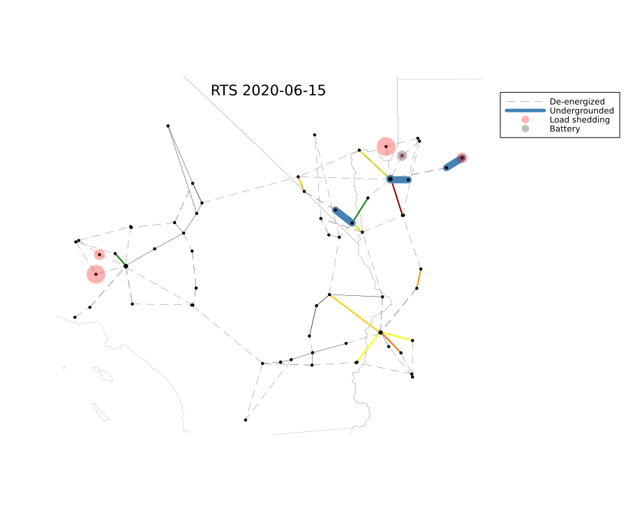

Network overview

4e. Tradeoff curve

Sweeping tradeoff_weight traces the Pareto front between load shedding and wildfire risk. Pass the vector of results to plot_results:

tradeoff_results = Dict[]
for w in [0.0, 0.25, 0.5, 0.75, 1.0]
    r = solve_ots(merge(SETTINGS, Dict(
        :network         => "RTS",
        :model           => "DCOTS",
        :objective       => "tradeoff",
        :tradeoff_weight => w,
        :times           => [(2020, 6, 15)],
    )))
    push!(tradeoff_results, r)
end

plot_results(tradeoff_results, [:tradeoff_curve];
             format="png", output_dir="tutorial_plots")

Loading RTS wildfire data from CSV...
Loaded RTS wildfire data from CSV for 1 days, max 90 risky lines per day
Building DCOTS model...
Switching method: optimal
Network: RTS
Objective: tradeoff
Days: 1, Hours per day: 6
Adding variables...
Adding objective function...
Adding constraints...
Solving optimization...
Extracting results...
Optimization complete!
Status: OPTIMAL
Objective value: -7.46836570484146e-16
Total load shed: -1.872946242542639e-13
Risk reduction: 70.77%
Total islanded buses: 52
Loading RTS wildfire data from CSV...
Loaded RTS wildfire data from CSV for 1 days, max 90 risky lines per day
Building DCOTS model...
Switching method: optimal
Network: RTS
Objective: tradeoff
Days: 1, Hours per day: 6
Adding variables...
Adding objective function...
Adding constraints...
Solving optimization...
Extracting results...
Optimization complete!
Status: OPTIMAL
Objective value: 0.0333976470360969
Total load shed: 2.4522744945798536e-13
Risk reduction: 86.64%
Total islanded buses: 60
Loading RTS wildfire data from CSV...
Loaded RTS wildfire data from CSV for 1 days, max 90 risky lines per day
Building DCOTS model...
Switching method: optimal
Network: RTS
Objective: tradeoff
Days: 1, Hours per day: 6
Adding variables...
Adding objective function...
Adding constraints...
Solving optimization...
Extracting results...
Optimization complete!
Status: OPTIMAL
Objective value: 0.05296252004420112
Total load shed: 14.084328960000056
Risk reduction: 95.02%
Total islanded buses: 61
Loading RTS wildfire data from CSV...
Loaded RTS wildfire data from CSV for 1 days, max 90 risky lines per day
Building DCOTS model...
Switching method: optimal
Network: RTS
Objective: tradeoff
Days: 1, Hours per day: 6
Adding variables...
Adding objective function...
Adding constraints...
Solving optimization...
Extracting results...
Optimization complete!
Status: OPTIMAL
Objective value: 0.04190773963008953
Total load shed: 32.35215769599937
Risk reduction: 98.71%
Total islanded buses: 64
Loading RTS wildfire data from CSV...
Loaded RTS wildfire data from CSV for 1 days, max 90 risky lines per day
Building DCOTS model...
Switching method: optimal
Network: RTS
Objective: tradeoff
Days: 1, Hours per day: 6
Adding variables...
Adding objective function...
Adding constraints...
Solving optimization...
Extracting results...
Optimization complete!
Status: OPTIMAL
Objective value: 0.0
Total load shed: 91.36595893512526
Risk reduction: 100.0%
Total islanded buses: 69
✓ Saved: tutorial_plots/tradeoff_curve.png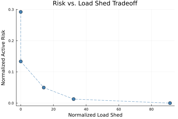

Tradeoff curve

5. Parameters and Customization

5a. Objective functions

`:objective`	Minimizes	Best for
`"loadshed"`	Total load shed (MW)	Reliability studies
`"wildfire"`	Active wildfire risk	Wildfire safety focus
`"cost"`	Generation cost + VOLL × load shed (+ investment costs)	Economic studies
`"tradeoff"`	Weighted shed + risk	Pareto analysis

results_cost = solve_ots(merge(SETTINGS, Dict(
    :network   => "RTS",
    :model     => "DCOTS",
    :objective => "cost",
    :voll      => 10000.0,           # $/MWh value of lost load
    :times     => [(2020, 6, 15)],
)));

println("Total cost: \$", round(results_cost[:objective_value], digits=0))

Loading RTS wildfire data from CSV...
Loaded RTS wildfire data from CSV for 1 days, max 90 risky lines per day
Building DCOTS model...
Switching method: optimal
Network: RTS
Objective: cost
Days: 1, Hours per day: 6
Adding variables...
Adding objective function...
Adding constraints...
Solving optimization...
Extracting results...
Optimization complete!
Status: OPTIMAL
Objective value: -5.551115123125783e-13
Total load shed: -5.551115123125783e-17
Risk reduction: 29.91%
Total islanded buses: 2
Total cost: $-0.0

5b. Multi-day studies

Pass several days (or a month/year string) and results arrays gain a day dimension [D × T × ...]. Investment decisions are shared across all days while operations are day-specific.

results_multi = solve_ots(merge(SETTINGS, Dict(
    :network   => "RTS",
    :model     => "DCOTS",
    :objective => "loadshed",
    :times     => [(2020, 6, 10), (2020, 6, 11), (2020, 6, 12)],
)));

println("Days solved: ", results_multi[:D])
println("Load shed by day: ",
        [round(sum(results_multi[:load_shedding][d, :, :]) * 100, digits=2) for d in 1:3], " MW")

Loading RTS wildfire data from CSV...
Loaded RTS wildfire data from CSV for 3 days, max 90 risky lines per day
Building DCOTS model...
Switching method: optimal
Network: RTS
Objective: loadshed
Days: 3, Hours per day: 6
Adding variables...
Adding objective function...
Adding constraints...
Solving optimization...
Extracting results...
Optimization complete!
Status: OPTIMAL
Objective value: 1.214306433183765e-16
Total load shed: 0.0
Risk reduction: 0.0%
Total islanded buses: 0
Days solved: 3
Load shed by day: [0.0, 0.0, 0.0] MW

5c. Solver settings

:optimizer  => HiGHS.Optimizer   # any JuMP MIP solver (default: Gurobi)
:mip_gap    => 0.001             # relative optimality gap (default 0.01)
:time_limit => 3600.0            # seconds (default 86400)
:silent     => true              # suppress solver log
:log_str    => "solve.log"       # write the Gurobi log to a file
:lp_str     => "model.lp"        # export the model as an LP file

5d. Saving and loading results

out = mktempdir()
solve_ots(merge(SETTINGS, Dict(
    :network       => "RTS",
    :model         => "DCOPF",
    :objective     => "loadshed",
    :times         => [(2020, 6, 15)],
    :output_format => "jld2",
    :output_path   => joinpath(out, "rts_base.jld2"),
)));

using JLD2
reloaded = JLD2.load(joinpath(out, "rts_base.jld2"), "results")
println("Reloaded load shed: ", round(reloaded[:total_load_shed], digits=2), " MW")

┌ Warning: solve_ots called with OPF-only model DCOPF; delegating to solve_opf. Prefer solve_opf for DCOPF/LACOPF.
└ @ PowerGridPlanning ~/work/PowerGridPlanning.jl/PowerGridPlanning.jl/src/PowerGridPlanning.jl:158
✓ OPF-only model (DCOPF): wildfire risk disabled
Building DCOPF model...
Switching method: optimal
Network: RTS
Objective: loadshed
Days: 1, Hours per day: 6
Adding variables...
Adding objective function...
Adding constraints...
Solving optimization...
Extracting results...
Optimization complete!
Status: OPTIMAL
Objective value: 0.0
Total load shed: 0.0
Risk reduction: 0.0%
Results saved to: /tmp/jl_F0qpse/rts_base.jld2
Reloaded load shed: 0.0 MW

5e. LACOTS: linearized AC model

LACOTS adds reactive power and voltage-magnitude variables for a more accurate AC representation. warm_start => "auto" first solves DCOTS and initializes LACOTS from it.

results_lac = solve_ots(merge(SETTINGS, Dict(
    :network    => "RTS",
    :model      => "LACOTS",
    :objective  => "loadshed",
    :times      => [(2020, 6, 15)],
    :warm_start => "auto",
)));

println("LACOTS load shed: ", round(results_lac[:total_load_shed], digits=2), " MW")

Loading RTS wildfire data from CSV...
Loaded RTS wildfire data from CSV for 1 days, max 90 risky lines per day
Running DC counterpart first for warm start...
Building DCOTS model...
Switching method: optimal
Network: RTS
Objective: loadshed
Days: 1, Hours per day: 6
Adding variables...
Adding objective function...
Adding constraints...
Solving optimization...
Extracting results...
Optimization complete!
Status: OPTIMAL
Objective value: 3.469446951953614e-18
Total load shed: 0.0
Risk reduction: 0.0%
Total islanded buses: 0
Building LACOTS model...
Switching method: optimal
Network: RTS
Objective: loadshed
Days: 1, Hours per day: 6
Adding variables...
Adding objective function...
Adding constraints...
Solving optimization...
Extracting results...
Optimization complete!
Status: OPTIMAL
Objective value: 5.204170427930421e-18
Total load shed: 0.0
Risk reduction: 0.0%
Total islanded buses: 0
LACOTS load shed: 0.0 MW

5f. Nonlinear AC verification

verify_ac replays fixed planning decisions in a full nonlinear AC model (via Ipopt): "ACPF" checks strict feasibility, "ACOPF" runs recovery redispatch with load shedding. Diagnostics are enabled by default and report solver failures, voltage violations, thermal overloads, angle-limit violations, recovery load shedding, reactive limit binding, and islanding.

mkpath("tutorial_output")

ac = verify_ac(Dict(
    :network  => "RTS",
    :mode     => "ACOPF",
    :times    => [(2020, 6, 15)],
    :T        => 1,                  # one hour keeps the tutorial fast
    :data_dir => "test_data",
    :feedback_enabled => true,
    :feedback_output_path => "tutorial_output/ac_diagnostic_report.md",
), results_thresh);

println("AC-feasible in all hours: ", ac[:feasible_all])
println("AC load shed: ", round(ac[:total_load_shed], digits=3))
println("Diagnostic counts: ", ac[:violation_summary][:count_by_type])
println("Diagnostic report: ", get(ac, :diagnostic_report_path, "none"))

✓ OPF-only model (DCOPF): wildfire risk disabled

******************************************************************************
This program contains Ipopt, a library for large-scale nonlinear optimization.
 Ipopt is released as open source code under the Eclipse Public License (EPL).
         For more information visit https://github.com/coin-or/Ipopt
******************************************************************************

AC-feasible in all hours: true
AC load shed: 0.482
Diagnostic counts: Dict(:active_load_shed => 1, :reactive_load_shed => 1, :islanding => 1)
Diagnostic report: tutorial_output/ac_diagnostic_report.md

5g. Custom wildfire risk data

Supply your own per-line risk instead of the built-in USGS FPI files, as a nested dictionary day_index => Dict(line_id => risk):

day_df = filter(r -> string(r.date_of_forecast) == "2020-06-15", rts_risk)
custom_risk = Dict(1 => Dict{Int,Float64}(
    row.branch_id => 2.0 * row.cum_wfpi for row in eachrow(day_df)))

results_custom = solve_ots(merge(SETTINGS, Dict(
    :network       => "RTS",
    :model         => "DCOTS",
    :objective     => "tradeoff",
    :tradeoff_weight => 0.5,
    :times         => [(2020, 6, 15)],
    :risk_per_line => custom_risk,
)));

println("Lines off under doubled risk: ", results_custom[:switched_off_lines][1])

✓ risk_per_line validation passed:
  - 1 days of data
  - 120 total line-day risk entries
  - Min/Max risky lines per day: 120/120
✓ Using user-provided risk_per_line data
Building DCOTS model...
Switching method: optimal
Network: RTS
Objective: tradeoff
Days: 1, Hours per day: 6
Adding variables...
Adding objective function...
Adding constraints...
Solving optimization...
Extracting results...
Optimization complete!
Status: OPTIMAL
Objective value: 0.05296252004420101
Total load shed: 14.084328959999999
Risk reduction: 95.02%
Total islanded buses: 72
Lines off under doubled risk: [1, 2, 3, 4, 5, 7, 8, 12, 13, 14, 18, 19, 20, 21, 23, 24, 27, 28, 29, 30, 31, 32, 33, 34, 35, 37, 38, 40, 41, 42, 43, 44, 45, 46, 48, 49, 50, 52, 53, 54, 55, 57, 59, 60, 62, 63, 66, 67, 68, 69, 71, 72, 73, 74, 75, 76, 78, 79, 80, 81, 82, 83, 84, 85, 86, 87, 88, 90, 91, 92, 93, 94, 96, 97, 99, 100, 101, 102, 103, 104, 105, 106, 107, 108, 109, 110, 111, 112, 113, 114, 115, 116, 117, 118, 119, 120]

5h. User-supplied networks

Any MATPOWER .m case can be used directly via :case_file — no pre-configuration needed. A bare case solves DCOPF/LACOPF out of the box; geography-dependent features ask explicitly for the data they need (see User-Supplied Networks in the Usage Guide). Here we treat the bundled RTS case file as if it were an external case:

my_case = joinpath(DATA, "networks", "RTS_GMLC.m")

results_file = solve_ots(merge(SETTINGS, Dict(
    :case_file => my_case,           # any path; :network label defaults to the file name
    :model     => "DCOPF",
    :objective => "loadshed",
    :times     => [(2020, 6, 15)],
)));

println("Solved network '", results_file[:network], "' from a case file path")

┌ Warning: solve_ots called with OPF-only model DCOPF; delegating to solve_opf. Prefer solve_opf for DCOPF/LACOPF.
└ @ PowerGridPlanning ~/work/PowerGridPlanning.jl/PowerGridPlanning.jl/src/PowerGridPlanning.jl:158
✓ Loaded user-supplied case file: /home/runner/work/PowerGridPlanning.jl/PowerGridPlanning.jl/test_data/networks/RTS_GMLC.m (label: RTS_GMLC)
✓ OPF-only model (DCOPF): wildfire risk disabled
Building DCOPF model...
Switching method: optimal
Network: RTS_GMLC
Objective: loadshed
Days: 1, Hours per day: 6
Adding variables...
Adding objective function...
Adding constraints...
Solving optimization...
Extracting results...
Optimization complete!
Status: OPTIMAL
Objective value: 0.0
Total load shed: 0.0
Risk reduction: 0.0%
Solved network 'RTS_GMLC' from a case file path

5i. Auto-plotting during solve

Set :plots to generate figures automatically at the end of solve_ots:

:plots    => "all",          # or "inv_only" / "timeseries_only"
:plot_dir => "my_plots",

Summary

Step	What you did
Setup	Loaded the package and the bundled reference dataset
Baseline	DCOPF with no switching — the minimal model
Switching	Thresholded heuristic vs. optimal MIP with the tradeoff objective
Investments	Hardening, batteries, and solar under one shared budget
Plots	Geographic overview, time series, and the Pareto tradeoff curve
Customization	Objectives, multi-day horizons, solver settings, saving/loading
Fidelity	LACOTS linearized AC and nonlinear AC verification with `verify_ac`
Your data	Custom risk dictionaries and user-supplied MATPOWER cases

For the full parameter reference, see the Usage Guide and API Reference.

This page was generated using Literate.jl.